The 2D Problem

The 2D Problem

Limitation of 2D

The diagram below the cross section of several 3D-shapes. If you presented just the cross section and were asked to guess what shape you could guess any of the three and depending on where we sectioned the shapes, we could also easily be confused as to the scale of the 3D volume.

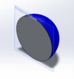
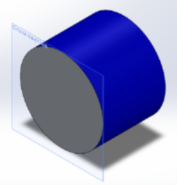
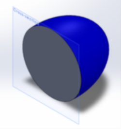
Fig 1: (left to right) cross sections of a sphere, cylinder and ellipsoid. Regardless of the 3D-shape, all three can give the same circular cross section.

Without context, a 2D cross-section can be misleading. This is an issue with traditional techniques in metallography and geology as microstructures can look very different when viewed from different directions; an example is from super-duplex stainless steel is illustrated here. Typically, a material is cut, polished and then only a section of the material is analysed, showing only part of the entire picture. Although this might be done in several orthogonal directions (as below) to provide more information this is not only time intensive, it also requires the sample to be destroyed, meaning no further testing can occur. Hercules offers a different option though, through a technique called Diffraction Contrast Tomography (DCT).

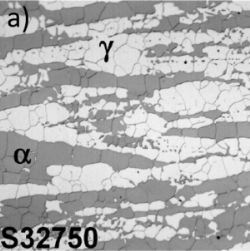
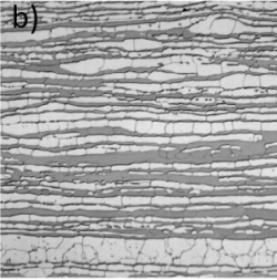
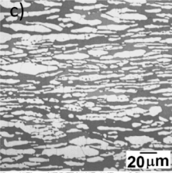
Fig 2: example optical micrographs from S32750 super-duplex stainless steel. Grains appear equiaxed when viewed in (a) cross-section normal to the rolling directions however, cross sections in the two rolling directions, (b) longitudinal and c) traverse directions, clearly show elongated grains.[1]

Why is Diffraction Contrast Tomography different from MicroCT?

Like medical x-rays, MicroCT is based on contrast caused by different materials absorbing different percentages of incident x-rays (Absorption Contrast Tomography) reducing the transmitted intensity. By rotating the sample, we get multiple projections allowing for a 3D-reconstruction of the sample.

This method alone isn’t very applicable if we wish to determine the microstructure of a single composition material.

Diffraction contrast tomography (DCT) is a non-destructive technique for the 3D characterisation of polycrystals containing up to a few thousand grains. While it is an established technique at synchrotrons ,  it is still an emerging technique for lab based x-ray sources which only becomes available,  as part of the ZEISS Hercules solution. When the sample rotates, some crystalline phases within the sample will fulfil the Bragg condition, meaning that some x-rays will be diffracted as well as absorbed. This gives both a dark spot in our transmitted image, indicating the real space position of the diffracting crystal, but also a diffraction pattern. By measuring the diffraction patterns at many angles and combining this with knowledge of the material being analysed, information about the orientation of the crystal can be  calculated  as well as the grain shape and size.

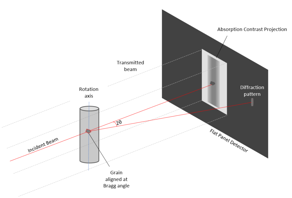
Fig 3: Schematic diagram of MicroCT and DCT technique.

Why use DCT rather than Electron Back Scatter Diffraction (EBSD)?

EBSD, while fantastic at giving us fine detail about orientation and engineering strain, relies on cross sections that are time consuming to prepare and only obtains part of the available information about the sample. While we could use 3D-EBSD to reconstruct a 3D-volume, the scale at which this is practical is much smaller than DCT and more importantly is destructive.

Moreover, as DCT is non-destructive, we can take more than just a single snapshot. A tensile (need to check with Zeiss, do they have a better example that shows sample at different stages?) specimen of Al-4wt%Cu is illustrated here with the measurement done with DCT. Not only can we see the grain orientation, shown in the Inverse Pole Figure colour (as in EBSD), but also we can take snapshots showing us the evolution of the grain structure. The X-ray setup at Hercules can apply loads up to 5kN as well as heating or cooling the sample while it is being scanned.

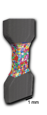
Fig 4: Diffraction Contrast Tomography map of Al-4wt%Cu tensile sample.

Correlating DCT and EBSD

Of course, if extra detail is required, Hercules also has further capability to take a region of interest identified in the DCT scan and prepare this for further EBSD studies, giving more localised information on orientation and strain within the sample. This multiscale approach provides both the wider context of the sample through its life time as well as the fine detail at the critical moments.

• [1]Modified from TF. Santos et al. Materials Research. 2016; 19(1): 117-131